Two-dimensional examples
Complete input files for 2D models using the dimensional and dimensionless streamfunction formulations are provided, for both isotropic and anisotropic porous media. These examples are provided in the Numbat examples folder.
Isotropic models
The first 2D examples are for an isotropic porous medium ().
Input file
The complete input file for this problem is
# 2D density-driven convective mixing
# The dimensional Numbat action is used to add all variables, kernels etc.
# Instability is seeded by small perturbation to porosity.
# A coarse grid and time stepping used to allow this model to run in ~ 15 minutes

[Mesh]
  type = NumbatBiasedMesh
  dim = 2
  nx = 150
  ny = 50
  ymax = 0.5
  refined_edge = top
  refined_resolution = 0.001
[]

[Numbat]
  [./Dimensional]
    concentration_scaling = 1e4
    boundary_concentration = 0.049306
    periodic_bcs = true
  [../]
[]

[AuxVariables]
  [./noise]
    family = MONOMIAL
    order = CONSTANT
  [../]
[]

[ICs]
  [./noise]
    type = RandomIC
    variable = noise
    max = 0.003
    min = -0.003
  [../]
  [./pressure]
    type = ConstantIC
    variable = pressure
    value = 10e6
  [../]
[]

[Materials]
  [./porosity]
    type = NumbatPorosity
    porosity = 0.3
    noise = noise
  [../]
  [./permeability]
    type = NumbatPermeability
    permeability = '1e-11 0 0 0 1e-11 0 0 0 1e-11'
  [../]
  [./diffusivity]
    type = NumbatDiffusivity
    diffusivity = 2e-9
  [../]
  [./density]
    type = NumbatDensity
    concentration = concentration
    zero_density = 994.56
    delta_density = 10.45
    saturated_concentration = 0.049306
  [../]
  [./viscosity]
    type = NumbatViscosity
    viscosity = 0.5947e-3
  [../]
[]

[Preconditioning]
  [./smp]
    type = SMP
    full = true
  [../]
[]

[Functions]
  [./timesteps]
    type = PiecewiseConstant
    x = '0 100 500 1e3 1e4 2e5'
    y = '10 50 100 500 1e3 1e3'
  [../]
[]

[Executioner]
  type = Transient
  l_max_its = 100
  end_time = 2e5
  solve_type = NEWTON
  petsc_options = -ksp_snes_ew
  petsc_options_iname = '-pc_type -sub_pc_type -ksp_atol'
  petsc_options_value = 'asm ilu 1e-12'
  nl_abs_tol = 1e-8
  [./TimeStepper]
    type = FunctionDT
    function = timesteps
  [../]
[]

[Outputs]
  perf_graph = true
  [./exodus]
    type = Exodus
    file_base = 2Dddc
    execute_on = 'INITIAL TIMESTEP_END'
  [../]
  [./csvoutput]
    type = CSV
    file_base = 2Dddc
    execute_on = 'INITIAL TIMESTEP_END'
  [../]
[]Running the example
This example can be run on the commandline using
numbat-opt -i 2Dddc.i
Alternatively, this file can be run using the Peacock gui provided by MOOSE using
peacock -i 2Dddc.i
in the directory where the input file 2Dddc.i resides.
Results
This 2D example should take only a few minutes to run to completion, producing a concentration profile similar to that presented in Figure 1, where several downwelling plumes of high concentration can be observed after 3528 s:
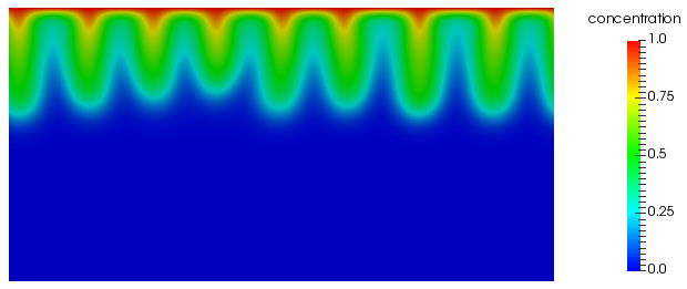
Figure 1: 2D concentration profile (t = 3528 s)
The flux per unit width over the top boundary is of particular interest in many cases (especially convective mixing of ). This is calculated using the boundaryfluxint postprocessor in the input file, and presented in \ref{fig:2Dflux}.
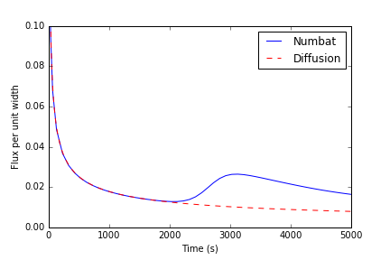
Figure 2: 2D flux across the top boundary
Initially, the flux is purely diffusive, and scales as , where is time (shown as the dashed red line). After some time, the convective instability becomes sufficiently strong, at which point the flux across the top boundary rapidly increases (at a time of approximately 2000 seconds).
Anisotropic models
The second 2D example is for an anisotropic porous medium with (ie., the vertical permeability is three quarters of the horizontal permeability).
Input file
# 2D density-driven convective mixing with permeability anisotropy gamma = 0.5
# The dimensional Numbat action is used to add all variables, kernels etc.
# Instability is seeded by small perturbation to porosity.
# A coarse grid and time stepping used to allow this model to run in ~ 15 minutes

[Mesh]
  type = NumbatBiasedMesh
  dim = 2
  nx = 150
  ny = 50
  ymax = 0.5
  refined_edge = top
  refined_resolution = 0.001
[]

[Numbat]
  [./Dimensional]
    concentration_scaling = 1e4
    boundary_concentration = 0.049306
    periodic_bcs = true
  [../]
[]

[AuxVariables]
  [./noise]
    family = MONOMIAL
    order = CONSTANT
  [../]
[]

[ICs]
  [./noise]
    type = RandomIC
    variable = noise
    max = 0.003
    min = -0.003
  [../]
  [./pressure]
    type = ConstantIC
    variable = pressure
    value = 10e6
  [../]
[]

[Materials]
  [./porosity]
    type = NumbatPorosity
    porosity = 0.3
    noise = noise
  [../]
  [./permeability]
    type = NumbatPermeability
    permeability = '1e-11 0 0 0 5e-12 0 0 0 1e-11'
  [../]
  [./diffusivity]
    type = NumbatDiffusivity
    diffusivity = 2e-9
  [../]
  [./density]
    type = NumbatDensity
    concentration = concentration
    zero_density = 994.56
    delta_density = 10.45
    saturated_concentration = 0.049306
  [../]
  [./viscosity]
    type = NumbatViscosity
    viscosity = 0.5947e-3
  [../]
[]

[Preconditioning]
  [./smp]
    type = SMP
    full = true
  [../]
[]

[Functions]
  [./timesteps]
    type = PiecewiseConstant
    x = '0 100 500 1e3 1e4 4e5'
    y = '10 50 100 500 1e3 2e3'
  [../]
[]

[Executioner]
  type = Transient
  l_max_its = 100
  end_time = 4e5
  solve_type = NEWTON
  petsc_options = -ksp_snes_ew
  petsc_options_iname = '-pc_type -sub_pc_type -ksp_atol'
  petsc_options_value = 'asm ilu 1e-12'
  nl_abs_tol = 1e-8
  [./TimeStepper]
    type = FunctionDT
    function = timesteps
  [../]
[]

[Outputs]
  perf_graph = true
  [./exodus]
    type = Exodus
    file_base = 2Dddc
    execute_on = 'INITIAL TIMESTEP_END'
  [../]
  [./csvoutput]
    type = CSV
    file_base = 2Dddc
    execute_on = 'INITIAL TIMESTEP_END'
  [../]
[]Note that the permeability anisotropy is introduced in the kernels using the gamma and anisotropic_tensor input parameters.
Running the example
This example can be run on the commandline using
numbat-opt -i 2Dddc_anisotropic.i
Alternatively, this file can be run using the Peacock gui provided by MOOSE using
peacock -i 2Dddc_anisotropic.i
in the directory where the input file 2Dddc_anisotropic.i resides.
Results
This 2D example should take only a few minutes to run to completion, producing a concentration profile similar to that presented in Figure 3, where several downwelling plumes of high concentration can be observed after 5000 s:
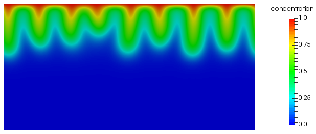
Figure 3: 2D concentration profile for (t = 5000 s)
In comparison to the isotropic example (with ) presented in Figure 1, we note that the concentration profile in the anisotropic example has only reached a similar depth after 5000 s (compared to 3528 s). The effect of the reduced vertical permeability in the anisotropic example slows the convective transport.
This observation can be quantified by comparing the flux per unit width over the top boundary of both examples, see Figure 4.
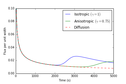
Figure 4: Comparison of the 2D flux across the top boundary
The inclusion of permeability anisotropy delays the onset of convection in comparison to the isotropic example, from a time of approximately 2000 seconds in the isotropic example to approximately 3500 seconds in the anisotropic example.