Three-dimensional examples
Complete input files for 2D models using the dimensional and dimensionless streamfunction formulations are provided, for both isotropic and anisotropic porous media. These examples are provided in the Numbat examples folder.
Isotropic models
The first examples are for an isotropic porous medium ().
Input file
The complete input file for this problem is
# 3D density-driven convective mixing. Instability is seeded by small perturbation
# to porosity. Don't try this on a laptop!

[Mesh]
  type = NumbatBiasedMesh
  dim = 3
  zmax = 1.5
  nx = 20
  ny = 20
  nz = 500
  refined_edge = front
  refined_resolution = 0.001
[]

[Numbat]
  [./Dimensional]
    concentration_scaling = 1e6
    boundary_concentration = 0.049306
    periodic_bcs = true
  [../]
[]

[AuxVariables]
  [./noise]
    family = MONOMIAL
    order = CONSTANT
  [../]
[]

[ICs]
  [./noise]
    type = RandomIC
    variable = noise
    max = 0.003
    min = -0.003
  [../]
  [./pressure]
    type = ConstantIC
    variable = pressure
    value = 1e6
  [../]
[]

[Materials]
  [./porosity]
    type = NumbatPorosity
    porosity = 0.3
    noise = noise
  [../]
  [./permeability]
    type = NumbatPermeability
    permeability = '1e-11 0 0 0 1e-11 0 0 0 1e-11'
  [../]
  [./diffusivity]
    type = NumbatDiffusivity
    diffusivity = 2e-9
  [../]
  [./density]
    type = NumbatDensity
    concentration = concentration
    zero_density = 995
    delta_density = 10.5
    saturated_concentration = 0.049306
  [../]
  [./viscosity]
    type = NumbatViscosity
    viscosity = 6e-4
  [../]
[]

[Preconditioning]
  [./smp]
    type = SMP
    full = true
  [../]
[]

[Executioner]
  type = Transient
  l_max_its = 200
  end_time = 3e5
  solve_type = NEWTON
  petsc_options = -ksp_snes_ew
  petsc_options_iname = '-pc_type -sub_pc_type -ksp_atol -pc_asm_overlap'
  petsc_options_value = 'asm ilu 1e-12 4'
  nl_abs_tol = 1e-10
  nl_max_its = 25
  dtmax = 2e3
  [./TimeStepper]
    type = IterationAdaptiveDT
    dt = 1
  [../]
[]

[Outputs]
  perf_graph = true
  [./exodus]
    type = Exodus
    file_base = 3Dddc
    execute_on = 'INITIAL TIMESTEP_END'
  [../]
  [./csvoutput]
    type = CSV
    file_base = 3Dddc
    execute_on = 'INITIAL TIMESTEP_END'
  [../]
[]Running the example
Examples of the total run times for this problem on a cluster are over 27 hours for a single processor down to only 30 minutes using 100 processors in parallel.
Results
This 3D example should produce a concentration profile similar to that presented in Figure 1, where several downwelling plumes of high concentration can be observed:
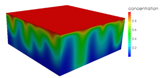
Figure 1: 3D concentration profile
Note that due to the random perturbation applied to the initial concentration profile, the geometry of the concentration profile obtained will differ from run to run.
The flux over the top surface is of particular interest in many cases (especially convective mixing of CO). This is calculated in this example file using the NumbatSideFlux in the input file, and presented in Figure 2.
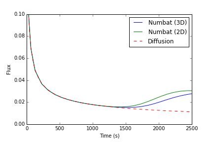
Figure 2: 3D flux across the top boundary
Initially, the flux is purely diffusive, and scales as , where is time (shown as the dashed green line). After some time, the convective instability becomes sufficiently strong, at which point the flux across the top boundary rapidly increases (at a time of approximately 1,700 seconds). Also shown for comparison is the flux for the 2D example. It is apparent that the 3D model leads in a slower onset of convection (the time where the flux first increases from the diffusive rate).
Large model
Increasing the size of the mesh enables more of the flow regimes to be modelled (at the cost of increased computational expense). Consider a dimensionless model with Rayleigh number . Lateral model dimensions are chosen so that approximately twenty fingers in the lateral directions are present at the onset of convection.
A suitable fully unstructured mesh for this model that is sufficiently refined near the top boundary with increasing element size with depth to minimise the number of elements can be constructed in an external meshing code. In this example, the open-source mesh generator Gmsh is used. The following geometry file describes the dimensions of the model and the target resolutions.
// Gmsh geometry file for a 3D mesh corresponding to
// Ra = 5000 (dimensionless model).
// The mesh is refined at the top boundary with element
// size increasing with depth.
//
// This geometry file can be converted to a mesh using
// gmsh -3 Ra5000.geo

// Mesh width in each dimension
xmax = 2000;
ymax = 2000;
zmax = 5000;

// Resolution at the top and bottom
lctop = 10;
lcbot = 200;

// Vertices of mesh
Point(1) = {0, 0, 0, lcbot};
Point(2) = {xmax, 0, 0, lcbot};
Point(3) = {0, ymax, 0, lcbot};
Point(4) = {xmax, ymax, 0, lcbot};
Point(5) = {xmax, ymax, zmax, lctop};
Point(6) = {xmax, 0, zmax, lctop};
Point(7) = {0, ymax, zmax, lctop};
Point(8) = {0, 0, zmax, lctop};

// Lines connecting vertices
Line(1) = {3, 7};
Line(2) = {7, 5};
Line(3) = {5, 4};
Line(4) = {4, 3};
Line(5) = {3, 1};
Line(6) = {2, 4};
Line(7) = {2, 6};
Line(8) = {6, 8};
Line(9) = {8, 1};
Line(10) = {1, 2};
Line(11) = {8, 7};
Line(12) = {6, 5};

// Surfaces defined by lines
Line Loop(13) = {7, 8, 9, 10};
Plane Surface(14) = {13};
Line Loop(15) = {6, 4, 5, 10};
Plane Surface(16) = {15};
Line Loop(17) = {3, 4, 1, 2};
Plane Surface(18) = {17};
Line Loop(19) = {12, -2, -11, -8};
Plane Surface(20) = {19};
Line Loop(21) = {7, 12, 3, -6};
Plane Surface(22) = {21};
Line Loop(23) = {9, -5, 1, -11};
Plane Surface(24) = {23};
Surface Loop(25) = {14, 22, 20, 18, 16, 24};

// Volume defined by surfaces
Volume(26) = {25};

// Make the sides suitable for periodic boundary conditions
Periodic Surface {18} = {14} Translate {0, ymax, 0};
Periodic Surface {22} = {24} Translate {xmax, 0, 0};

// Name the faces for easy application of boundary conditions
Physical Surface("top") = {20};
Physical Surface("bottom") = {16};
Physical Surface("front") = {14};
Physical Surface("back") = {18};
Physical Surface("left") = {24};
Physical Surface("right") = {22};
Physical Volume("0") = {26};This mesh geometry file can be used to generate a mesh using Gmsh, either through its graphical user interface, or alternatively, on the commandline
gmsh -3 Ra5000.geo
which results in a mesh file with approximately 8.4 million tetrahedral elements.
Input file
The complete input file for this problem is
# Density-driven convective mixing in a 3D model using the streamfunction
# formulation for Ra = 5000
#
# Uses an unstructured mesh generated by Gmsh
# To generate the mesh, run 'gmsh -3 Ra5000.geo'
#
# Note: this mesh has approximately 8.4 million elements and takes about
# 8 hours to run using 200 processors

[Mesh]
  type = FileMesh
  file = Ra5000.e
[]

[Numbat]
  [./Dimensionless]
  [../]
[]

[ICs]
  [./concentration]
    type = NumbatPerturbationIC
    variable = concentration
    amplitude = 0.1
    seed = 1
  [../]
  [./streamfunctionx]
    type = ConstantIC
    variable = streamfunction_x
    value = 0.0
  [../]
  [./streamfunctiony]
    type = ConstantIC
    variable = streamfunction_y
    value = 0.0
  [../]
[]

[Functions]
  [./timesteps]
    type = PiecewiseConstant
    x = '0 10 500 1e3 1e4 6e4'
    y = '9 10 50 100 200 200'
  [../]
[]

[Executioner]
  type = Transient
  end_time = 6e4
  start_time = 1
  solve_type = NEWTON
  petsc_options = -snes_ksp_ew
  petsc_options_iname = '-ksp_type -pc_type -pc_asm_overlap -sub_pc_type -pc_factor_levels -ksp_atol'
  petsc_options_value = 'gmres asm 10 ilu 4 1e-12'
  nl_abs_tol = 1e-9
  l_max_its = 200
  [./TimeStepper]
    type = FunctionDT
    function = timesteps
  [../]
[]

[Preconditioning]
  [./smp]
    type = SMP
    full = true
  [../]
[]

[Outputs]
  perf_graph = true
  [./exodus]
    type = Exodus
    execute_on = 'INITIAL TIMESTEP_END'
    interval = 4
  [../]
  [./csvoutput]
    type = CSV
    execute_on = 'INITIAL TIMESTEP_END'
  [../]
  [./checkpoint]
    type = Checkpoint
    num_files = 2
    interval = 10
  [../]
[]An example of the evolution of the convective fingers in this model are presented in Figure 3 and Figure 4 for an isotropic model. The concentration profile just after the onset of convection is shown in Figure 3 for a dimensionless time . As the isosurface shows, there are a large number of small fingers at this stage. As time increases, these small structures merge, forming larger fingers in a process that continues as time proceeds, until only a few large fingers are present, see Figure 4. This merging behaviour is very complicated and difficult to characterise in any quantitative manner
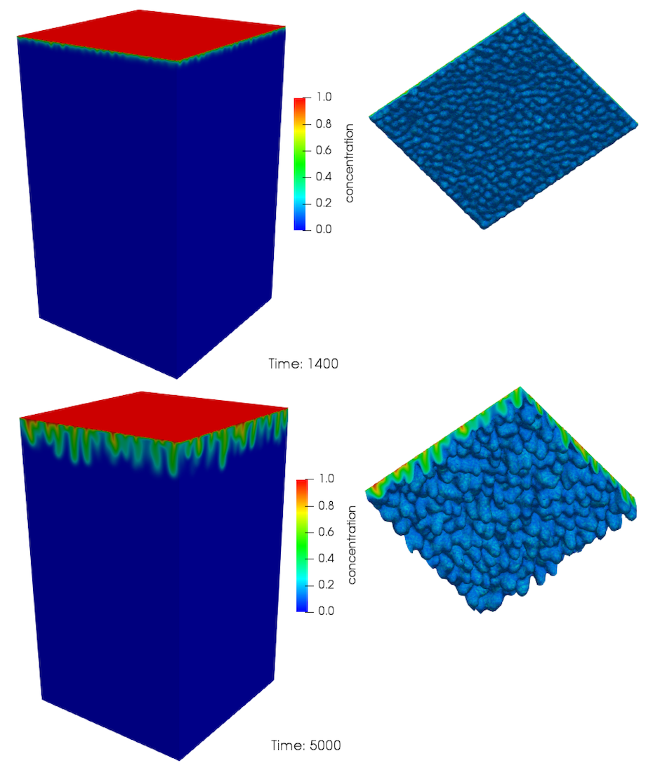
Figure 3: Evolution of convective mixing in 3D. Time is dimensionless.
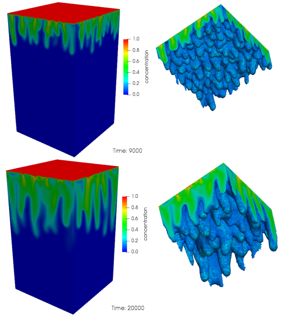
Figure 4: Evolution of convective mixing in 3D (continued). Time is dimensionless.
Many interesting observations can be made from large-scale 3D models. For example, the temporal evolution of the fingers shown in Figure 3 and Figure 4 can also be examined through a horizontal slice through the model, see Figure 5. In this example, a horizontal slice is taken at a dimensionless distance of 100 from the top surface (where the CO concentration is 1). As the fingers approach this depth, they are initially observed as circular regions of higher concentration, cf Figure 5 (a) and (b), where we can see that the fingers have just reached this depth at dimensionless time 1000. As time increases, the complexity of the fingering process can be observed, with merging of adjacent fingers and growth observed. Like Pau et al. (2010) and Fu et al. (2013), we observe that the fingers arrange themselves into polygonal structures with thin profiles surrounded by large regions of unsaturated fluid, see Figure 5 (d), (e) and (f).
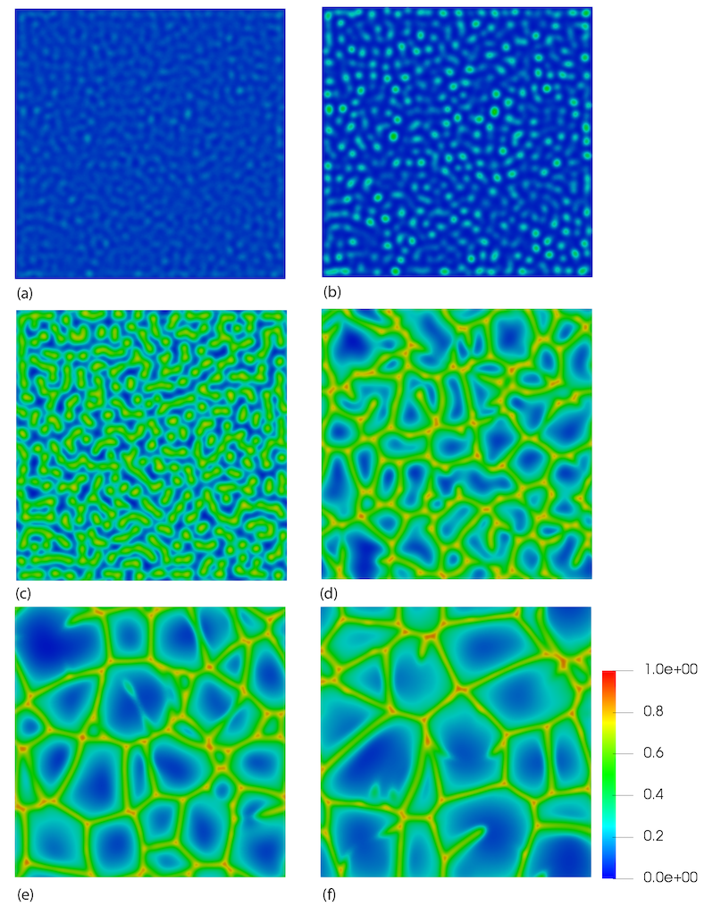
Figure 5: Horizontal slice at dimensionless depth 10 showing the evolution of the convective fingers in 3D. Time increasing from (a) to (f).
References
- Xiaojing Fu, Luis Cueto-Felgueroso, and Ruben Juanes.
Pattern formation and coarsening dynamics in three-dimensional convective mixing in porous media.
Phil. Trans. R. Soc. A, 371:20120355, 2013.[BibTeX]
- George SH Pau, John B Bell, Karsten Pruess, Ann S Almgren, Michael J Lijewski, and Keni Zhang.
High-resolution simulation and characterization of density-driven flow in CO$_2$ storage in saline aquifers.
Advances in Water Resources, 33:443–455, 2010.[BibTeX]