Polynomial Fitting
To introduce the idea of finding coefficients to functions, let's consider simple polynomial fitting.
In polynomial fitting (or interpolation) you have a set of points and you are looking for the coefficients to a function that has the form:
Where a, b and c are scalar coefficients and 1, x, x^2 are "basis functions".
Find a, b, c, etc. such that f(x) passes through the points you are given.
More generally you are looking for: where the c_i are coefficients to be determined.
f(x) is unique and interpolary if d+1 is the same as the number of points you need to fit.
Need to solve a linear system to find the coefficients.
Example
Define a set of points:
Substitute data into the model:
Leads to the following linear system for , , and :
Solving for the coefficients results in:
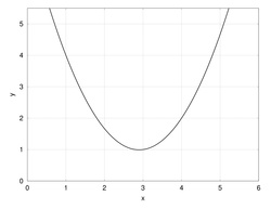
These define the solution function:
Important! The solution is the function, not the coefficients.
The coefficients themselves don't mean anything, by themselves they are just numbers.
The solution is not the coefficients, but rather the function they create when they are multiplied by their respective basis functions and summed.
The function does go through the points we were given, but it is also defined everywhere in between.
We can evaluate at the point , for example, by computing: or more generically: where the correspond to the coefficients in the solution vector, and the are the respective functions.
Finally, note that the matrix consists of evaluating the functions at the points.
Finite Elements Simplified
A method for numerically approximating the solution to Partial Differential Equations (PDEs).
Works by finding a solution function that is made up of "shape functions" multiplied by coefficients and added together.
Just like in polynomial fitting, except the functions aren't typically as simple as (although they can be).
The Galerkin Finite Element method is different from finite difference and finite volume methods because it finds a piecewise continuous function which is an approximate solution to the governing PDE.
Just as in polynomial fitting you can evaluate a finite element solution anywhere in the domain.
You do it the same way: by adding up "shape functions" evaluated at the point and multiplied by their coefficient.
FEM is widely applicable for a large range of PDEs and domains.
It is supported by a rich mathematical theory with proofs about accuracy, stability, convergence and solution uniqueness.
Weak Form
Using FE to find the solution to a PDE starts with forming a "weighted residual" or "variational statement" or "weak form". - We typically refer to this process as generating a Weak Form.
The idea behind generating a weak form is to give us some flexibility, both mathematically and numerically.
A weak form is what you need to input to solve a new problem.
Generating a weak form generally involves these steps:
Write down strong form of PDE.
Rearrange terms so that zero is on the right of the equals sign.
Multiply the whole equation by a "test" function .
Integrate the whole equation over the domain .
Integrate by parts (use the divergence theorem) to get the desired derivative order on your functions and simultaneously generate boundary integrals.
Refresher: The divergence theorem
Transforms a volume integral into a surface integral:
Slight variation: multiply by a smooth function, :
In finite element calculations, for example with , the divergence theorem implies:
We often use the following inner product notation to represent integrals since it is more compact:
Example: Convection Diffusion
Write the strong form of the equation:
Rearrange to get zero on the right-hand side:
Multiply by the test function :
Integrate over the domain :
Apply the divergence theorem to the diffusion term:
Write in inner product notation. Each term of the equation will inherit from an existing MOOSE type as shown below.